Regular feed-forward artificial neural networks (ANN), like the type featured below, allow us to learn higher order non-linear features, which typically results in improved prediction accuracy over smaller models like logistic regression.
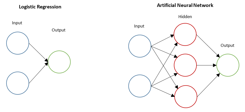
However, artificial neural networks have a number of problems that make them less ideal for certain types of problems. For example, imagine a case where we wanted to classify images of handwritten digits. An image is just a 2D array of pixel intensity values, so a small 28×28 pixel image has a total of 784 pixels. If we wanted to classify this using an ANN, we would flatten the 2D array into a 1D vector of size 784 and treat each pixel as a separate input neuron. So for a small image, we already have almost 1000 parameters to learn, and that is just for a single layer. To make things worse, images also contain three separate colour channels, so we actually have 3x as many input neurons per image. As input images approach more realistic sizes, the parameter count becomes very large.
ANNs also assume feature independence. This assumption is generally not tenable in most real world data and can hurt the performance of the model. In the context of images, this assumption states that the input features (i.e. the individual pixels) are unrelated to each other. However, this is not the case with the vast majority of images because pixels that are close each other likely belong to the same object/visual structure and should be treated similarly. There is nothing in the architecture of an ANN that allows that proximity to be learned, or at least accounted for.
These issues (along with many others) mean image classification problems are typically handled with Convolutional Neural Networks (CNN).
While still feedforward in nature, convolutional neural networks use a different network architecture to ANNs, and use kernel convolution as the primary operation. There are two additional layer types that need to be considered with a CNN: convolution and pooling.
Convolution layers
Convolution layers convolve a kernel over some input to produce a feature map (sometimes called an activation map):
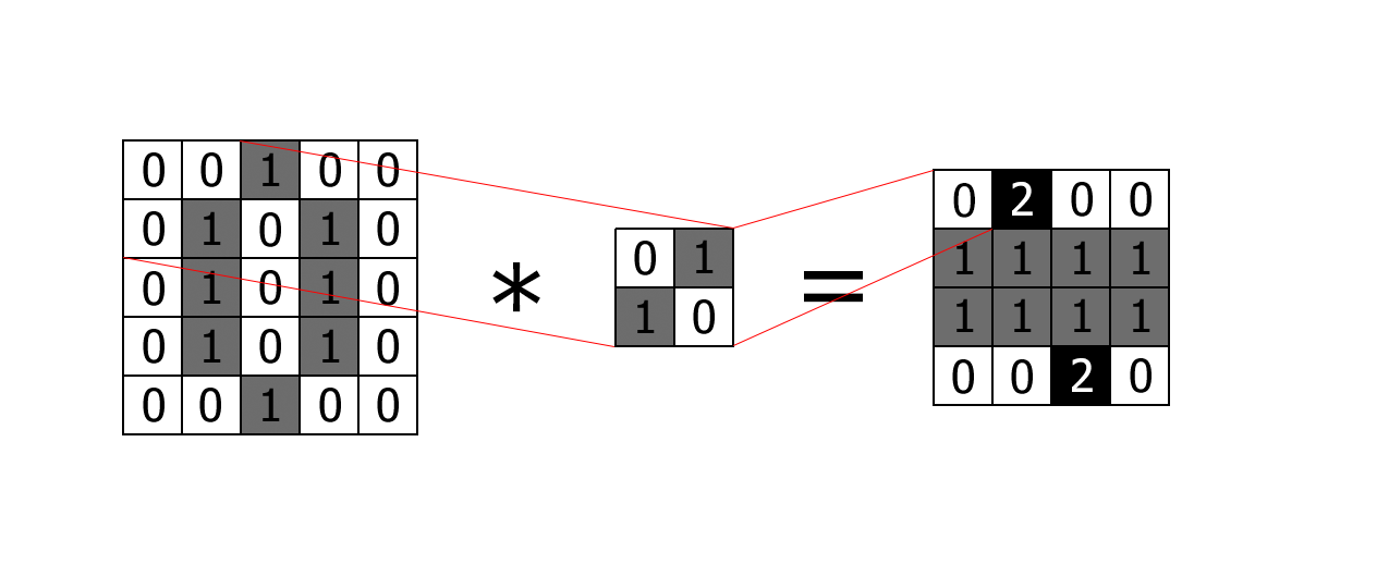
Imagine we were classifying grayscale hand written digits of size 5×5. The input would be a 2D array containing the pixel intensity values. We then specify a kernel of a particular size (2×2 in this case) and convolve it over the input to produce a 4×4 feature map as the output. This output feature map is then passed (as input) into the next layer. Convolution will reduce the size of the input unless we pad the input with 0 values (which we didn’t do in the example above).
A CNN, like other architectures previously discussed, is learning a set of weights. The weights in this case are the parameter values within the kernels. In essence, the network is learning the best kernel for separating the classes. There are a number of hyper parameters for a convolution layer:
- Number of kernels, which produce the same number of feature maps. In the example above we only have 1 kernel, which produces 1 feature map.
- Kernel size
- Stride, which is the number of spatial steps to move the kernel during convolution. Stride 1 will move the kernel 1 pixel at a time. Stride 2 will skip every other pixel.
- Padding, which is typically used to control the size of the feature map.
It is extremely important to note that the inputs and kernels are typically 3-dimensional. If the above input was a colour image, its size would be 5x5x3. The kernel always has the same depth as the input it is convolving over, so in the example the kernel would be 2x2x3. In other words, the kernel learns 3 2×2 spatial filters, one for each input channel. Each spatial filter contains a different set of weights. Finally, convolving a 3D kernel over a 3D input volume will produce a single 2D feature map.
To drive the point home:
- Input: 5x5x3 colour images
- 10 3×3 kernels (given the 3 channels of the input, each kernel is actually 3x3x3)
- Convolution produces the same number of feature maps as there are kernels, so we get 10 different 4×4 feature maps
- This 4x4x10 volume is then passed onto the next layer (if we stacked 2 convolution layers together, this volume is treated in the same way as the original 5x5x3 image, only with a smaller spatial extent and more depth channels)
ANN treats each image pixel as a separate neuron with its own parameter to be learned. Convolution layers allow the entire image to share the same kernel parameters, which drastically reduces the parameter count. Furthermore, the inputs are not treated independently (like in an ANN) because a kernel is looking at a number of surrounding pixels simultaneously. This allows the network to learn spatial structure. Of course, the input doesn’t have to be an image. If the input was time series data, for example, the kernel would be learning temporal structure instead.
Pooling layers
A pooling layer down samples any volume that it receives. If we took the convolution layer in the figure above and passed it directly into a pooling layer, then we get the following:
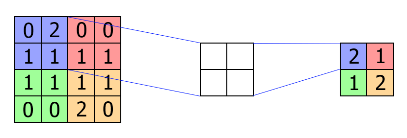
We choose a (parameter-less) kernel of a particular size and a stride (2×2 kernel with stride 2 in this example). Max-pooling is the most common form of pooling in CNNs. As we stride the kernel over the input, we simply take the maximum value within the kernel and set it as the output value. In the figure above you can see we’ve reduced the input size by half, which reduces the memory footprint of the rest of the network.
Note: Pooling is done separately for each depth slice of the (typically) 3D input volume.
Fully connected layers
Finally, fully connected layers are typically added to CNN architectures. This is the same fully connected layer type that can be found in traditional ANNs. It flattens the entire input volume into a single vector. Each element is treated as a separate input neuron. If we stack multiple layers together then we have the ANN architecture. Fully connected layers are typically placed at the end of a network and connects to the classifier layer for prediction.
The full CNN architecture stacks convolution, pooling, and fully connected layers, and in future posts we’ll see how everything comes together in Python to help us classify images.