Previously, we talked about simple OR gates and now we’ll continue that discussion with AND gates, and specifically the role of bias units. We often neglect to consider the role bias plays in our models. We know that we should include bias units, but why? Here, I’ll walk through a short example using an AND gate to highlight the importance of the bias unit.
Bias units allow us to offset the model in the same way that an intercept allows us to offset a regression line.
Imagine a simple AND gate. It will only fire if both inputs are true:
| Input 1 | Input 2 | Output |
|---|---|---|
| 0 | 0 | 0 |
| 0 | 1 | 0 |
| 1 | 0 | 0 |
| 1 | 1 | 1 |
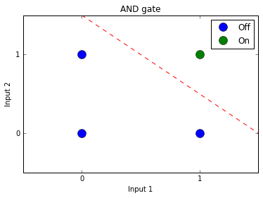
This relationship can be visualized like this:

As you can see from the plot, the linear separator cannot both cross the origin (0,0) and correctly split the categories, so we need to add a bias unit to offset the model.
What would happen if we omitted the bias unit? The following code creates a logistic regression model without bias (2 inputs, 1 output, sigmoid activation):
# Set inputs and correct output values
inputs = [[0,0], [1,1], [0,1], [1,0]]
outputs = [0, 1, 0, 0]

# Set training parameters
alpha = 0.1 # Learning rate
training_iterations = 30000

# Define tensors
x = T.matrix("x")
y = T.vector("y")

# Set random seed
rng = np.random.RandomState(2345)

# Initialize random weights
w_values = np.asarray(rng.uniform(low=-1, high=1, size=(2, 1)),
                      dtype=theano.config.floatX)
w = theano.shared(value=w_values, name='w', borrow=True)

# Theano symbolic expressions
hypothesis = T.nnet.sigmoid(T.dot(x, w)) # Sigmoid activation
hypothesis = T.flatten(hypothesis) # This needs to be flattened
                                   # so hypothesis (matrix) and
                                   # y (vector) have same shape

cost = T.nnet.binary_crossentropy(hypothesis, y).mean()
updates_rules = [
    (w, w - alpha * T.grad(cost, wrt=w))
]

# Theano compiled functions
train = theano.function(inputs=[x, y], outputs=[hypothesis, cost],
                        updates=updates_rules)
predict = theano.function(inputs=[x], outputs=[hypothesis])

# Training
cost_history = []

for i in range(training_iterations):
    h, cost = train(inputs, outputs)
    cost_history.append(cost)

# Plot training curve
plt.plot(range(1, len(cost_history)+1), cost_history)
plt.grid(True)
plt.xlim(1, len(cost_history))
plt.ylim(0, max(cost_history)+0.1)
plt.title("Training Curve")
plt.xlabel("Iteration #")
plt.ylabel("Cost")
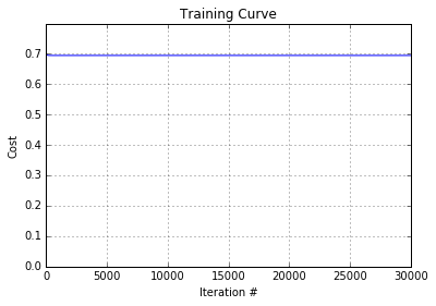
The training curve below shows that gradient descent is not able to converge on appropriate parameter values due to the lack of a bias unit:

As a result, the model makes incorrect predictions of 0.5 for the test data:
# Predictions
test_data = [[1,1], [1,1], [1,1], [1,0]]
predictions = predict(test_data)
print predictions

[0.5, 0.5, 0.5, 0.5]
The correct model for an AND gate must include a bias unit to offset the separator, and can be implemented as follows:
# Set inputs and correct output values
inputs = [[0,0], [1,1], [0,1], [1,0]]
outputs = [0, 1, 0, 0]

# Set training parameters
alpha = 0.1 # Learning rate
training_iterations = 30000

# Define tensors
x = T.matrix("x")
y = T.vector("y")
b = theano.shared(value=1.0, name='b') # Add bias unit

# Set random seed
rng = np.random.RandomState(2345)

# Initialize random weights
w_values = np.asarray(rng.uniform(low=-1, high=1, size=(2, 1)),
                      dtype=theano.config.floatX)
w = theano.shared(value=w_values, name='w', borrow=True)

# Theano symbolic expressions
hypothesis = T.nnet.sigmoid(T.dot(x, w) + b) # Sigmoid activation
hypothesis = T.flatten(hypothesis) # This needs to be flattened
                                   # so hypothesis (matrix) and
                                   # y (vector) have same shape

cost = T.nnet.binary_crossentropy(hypothesis, y).mean()
updates_rules = [
    (w, w - alpha * T.grad(cost, wrt=w)),
    (b, b - alpha * T.grad(cost, wrt=b))
]

# Theano compiled functions
train = theano.function(inputs=[x, y], outputs=[hypothesis, cost],
                        updates=updates_rules)
predict = theano.function(inputs=[x], outputs=[hypothesis])

# Training
cost_history = []

for i in range(training_iterations):
    h, cost = train(inputs, outputs)
    cost_history.append(cost)

# Plot training curve
plt.plot(range(1, len(cost_history)+1), cost_history)
plt.grid(True)
plt.xlim(1, len(cost_history))
plt.ylim(0, max(cost_history))
plt.title("Training Curve")
plt.xlabel("Iteration #")
plt.ylabel("Cost")
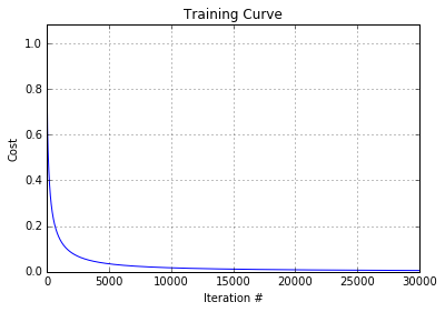
The training curve shows that gradient descent now converges correctly:

And we get correct predicted values:
# Predictions
test_data = [[1,1], [1,1], [1,1], [1,0]]
predictions = predict(test_data)
print predictions

[0.99999995, 0.99999995, 0.99999995, 0.00001523]
Bias units are typically added to machine learning models, and AND gates are a simple way of highlighting why they are important.
The full code can be found in my GitHub repo here (no bias) and here (with bias).