Theano is a powerful Python library that provides some useful tools for machine learning, such as GPU training and symbolic differentiation of the cost function during gradient descent.
It can be a bit challenging to understand how Theano works, so before jumping into more complex non-linear models, we can get to grips with Theano by implementing something simple like an OR gate.
An OR gate receives 2 inputs and will output true if either of the inputs are true. So, there are 3 cases where an OR gate will output a true value:
| Input 1 | Input 2 | Output |
|---|---|---|
| 0 | 0 | 0 |
| 0 | 1 | 1 |
| 1 | 0 | 1 |
| 1 | 1 | 1 |
We can also represent the problem visually:
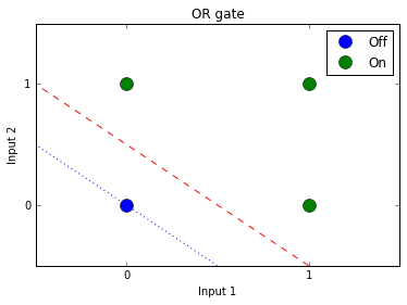
The goal is to create a model that receives 2 inputs and outputs 1 value. The model will learn a linear separator that can split the 2 output categories. Looking at the plot above, the red line is an ideal separator as it maximizes the margins between the categories. However, the blue line can also work as a separator, with one of the classes falling directly on it.
I won’t go into installing/setting up Theano here as there are many good guides on the topic (see here and here). However, in order to utilize a GPU during training we need to include the device flag and set float values to 32bit in the .theanorc file (typically found in your home directory):
floatX = float32
device = gpu
We’ll begin by importing some modules:
import numpy as np
import theano
import theano.tensor as T
import matplotlib.pyplot as plt
Next, we provide the training examples and the correct output labels. There are only 4 possible input combinations:
# Set inputs and correct output values
inputs = [[0,0], [1,1], [0,1], [1,0]]
outputs = [0, 1, 1, 1]
Set the learning rate and number of training iterations for batch gradient descent:
# Set training parameters
alpha = 0.1 # Learning rate
training_iterations = 30000
In Theano, we first have to define symbols that represent each variable (x and y) and their type (matrix and vector). b is a shared variable used by multiple functions and contains the model bias value:
# Define tensors
x = T.matrix("x")
y = T.vector("y")
b = theano.shared(value=1.0, name='b')
Next, we need to randomly initialize the weights. We do this by creating a numpy array with dimensions (2,1) containing random values sampled from a uniform distribution. The data type is set to float32 as defined in the .theanorc config file.
We can (optionally) set a random seed for reproducible results:
# Set random seed
rng = np.random.RandomState(2345)

# Initialize random weights
w_values = np.asarray(rng.uniform(low=-1, high=1, size=(2, 1)),
                      dtype=theano.config.floatX) # 32bit float for GPU

w = theano.shared(value=w_values, name='w', borrow=True)
Next, we have to define expressions that tell Theano how to evaluate things like the hypothesis and cost values using the symbols/tensors we defined earlier.
For example, the first line below calculates the dot product of the variables (x) and weights (w), adds the bias (b) term, and wraps the result in a sigmoid activation function. This is basically a logistic regression model.
It is important to note that no values are actually calculated at this stage. We are simply telling Theano how these values are calculated.
We’ll use binary cross entropy as the cost function. One advantage of Theano is that it can differentiate the function for us automatically.
The update_rules are used during gradient descent and tells Theano how to adjust the w and b values during back propagation. It is during this stage that we ask for the gradient (T.grad()) of the cost function with respect to the different parameters:
# Theano symbolic expressions
hypothesis = T.nnet.sigmoid(T.dot(x, w) + b) # Sigmoid activation
hypothesis = T.flatten(hypothesis) # This needs to be flattened
                                   # so hypothesis (matrix) and
                                   # y (vector) have same shape

cost = T.nnet.binary_crossentropy(hypothesis, y).mean() # CE

updates_rules = [
    (w, w - alpha * T.grad(cost, wrt=w)),
    (b, b - alpha * T.grad(cost, wrt=b))
]
Now that we’ve defined expressions and Theano knows how to calculate various values, we need to create some functions that can make use of those expressions.
During training, we need to evaluate the hypothesis and cost expressions, so we set those as the outputs for the train function. The inputs are the non-shared symbols/tensors required by those expressions (x and y). We also tell the function how parameters should be updated by passing in our update_rules:
# Theano compiled functions
train = theano.function(inputs=[x, y], outputs=[hypothesis, cost],
                        updates=updates_rules)

predict = theano.function(inputs=[x], outputs=[hypothesis])
Once our expressions and functions are in place, training is pretty straightforward. We loop over a number of training_iterations, and within each loop we call the train() function and pass in the inputs and outputs we defined earlier.
This step is where the bulk of the work happens. The model parameters/weights are adjusted after each iteration, converging on values that provide the best linear separator for our 2 classes.
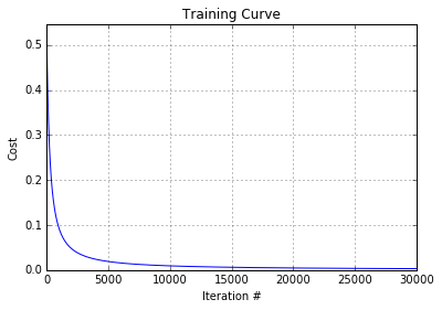
We can optionally append the cost of each iteration to a list so we can plot a training curve later:
# Training
cost_history = []

for i in range(training_iterations):
    h, cost = train(inputs, outputs)
    cost_history.append(cost)
Plotting a training curve is as simple as plotting the cost value after each iteration of training. The plot shows that gradient descent is converging correctly:
# Plot training curve
plt.plot(range(1, len(cost_history)+1), cost_history)
plt.grid(True)
plt.xlim(1, len(cost_history))
plt.ylim(0, max(cost_history))
plt.title("Training Curve")
plt.xlabel("Iteration #")
plt.ylabel("Cost")
Finally, we can use the predict() function we defined earlier to test the accuracy of our trained model. For the following test data, an OR gate should return values of [1, 1, 1, 1]:
# Predictions
test_data = [[1,1], [1,1], [1,1], [1,0]]
predictions = predict(test_data)
print predictions

[0.99999995,0.99999995,0.99999995,0.99729306]
The full code can be found in my GitHub repo here