Following my overview of Convolutional Neural Networks (CNN) in a previous post, now lets build a CNN model to 1) classify images of handwritten digits, and 2) see what is learned by this type of model. Handwritten digit recognition is the ‘Hello World’ example of the CNN world. I’ll be using the MNIST database of handwritten digits, which you can find here. The MNIST database contains grey scale images of size 28×28 (pixels), each containing a handwritten number from 0-9 (inclusive). The goal: given a single image, how do we build a model that can accurately recognize the number that is shown?
Let’s take a moment to consider how this model might work. The numbers from 0-9 look different and have different features: some contain only straight edges (e.g. 4) , some contain rounded edges (e.g. 5), and others have enclosed spaces (e.g. 8). A CNN is an ideal model for this problem because it can learn these different feature types and detect their presence/location in an image. We don’t need to be explicit about what features are important (often times we don’t know what features are important) – these so-called kernels will be learned by our model.
For this example I’ll be using the Lasagne package in Python. Lasagne is a library that allows us to build and train neural networks using Theano, and allows us to avoid a lot of the plumbing required to pass data around the layers of the network. If you’re interested in this plumbing, Michael Nielsen wrote a great module containing classes for the different layer types that’ll we need, which you can find here. In this post I’ll mainly be breaking down the Lasagne tutorial, but with a few additions. The code below is primarily from their tutorial
Loading the data
To begin, let’s get some imports out of the way:
from __future__ import print_function

import lasagne
import matplotlib.pyplot as plt
import numpy as np
import os
import sys
import theano
import theano.tensor as T
import time

from pylab import cm, imshow, show
Now, let’s import the MNIST data. The following function will download the data from Yann LeCun’s website and split the data into a train and test sets (along with their labels):
def load_dataset():
    # We first define a download function, supporting both Python 2 and 3.
    if sys.version_info[0] == 2:
        from urllib import urlretrieve
    else:
        from urllib.request import urlretrieve

    def download(filename, source='http://yann.lecun.com/exdb/mnist/'):
        print("Downloading %s" % filename)
        urlretrieve(source + filename, filename)

    # We then define functions for loading MNIST images and labels.
    # For convenience, they also download the requested files if needed.
    import gzip

    def load_mnist_images(filename):
        if not os.path.exists(filename):
            download(filename)
        # Read the inputs in Yann LeCun's binary format.
        with gzip.open(filename, 'rb') as f:
            data = np.frombuffer(f.read(), np.uint8, offset=16)
        # The inputs are vectors now, we reshape them to monochrome 2D images,
        # following the shape convention: (examples, channels, rows, columns)
        data = data.reshape(-1, 1, 28, 28)
        # The inputs come as bytes, we convert them to float32 in range [0,1].
        # (Actually to range [0, 255/256], for compatibility to the version
        # provided at http://deeplearning.net/data/mnist/mnist.pkl.gz.)
        return data / np.float32(256)

    def load_mnist_labels(filename):
        if not os.path.exists(filename):
            download(filename)
        # Read the labels in Yann LeCun's binary format.
        with gzip.open(filename, 'rb') as f:
            data = np.frombuffer(f.read(), np.uint8, offset=8)
        # The labels are vectors of integers now, that's exactly what we want.
        return data

    # We can now download and read the training and test set images and labels.
    X_train = load_mnist_images('train-images-idx3-ubyte.gz')
    y_train = load_mnist_labels('train-labels-idx1-ubyte.gz')
    X_test = load_mnist_images('t10k-images-idx3-ubyte.gz')
    y_test = load_mnist_labels('t10k-labels-idx1-ubyte.gz')

    # We reserve the last 10000 training examples for validation.
    X_train, X_val = X_train[:-10000], X_train[-10000:]
    y_train, y_val = y_train[:-10000], y_train[-10000:]

    # We just return all the arrays in order, as expected in main().
    return X_train, y_train, X_val, y_val, X_test, y_test
To load the data, simply call the function:
X_train, y_train, X_val, y_val, X_test, y_test = load_dataset()
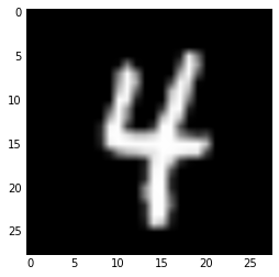
We can take a quick look at a random MNIST image to get a sense of what we’re working with:
image_num = np.random.randint(0, X_train.shape[0])
image_array = X_train[image_num][0]
image_2d = np.reshape(image_array, (28, 28))

imshow(image_2d, cmap=cm.gray)
Training the CNN
The first thing we need to do is define the architecture of the network. We can do that using Lasagne layers.
The following function defines the model architecture (note that the output of one layer is passed as input into the next layer):
- Input layer that accepts a 4D tensor containing our input image
- The first index is the mini-batch index, second index is the number of channels (1 channel for grey scale images), and finally we have the width and height of the input
- Convolution layer with 32 5×5 kernels followed by ReLU activation. It is common to use a rectifier as the activation function instead of the traditional sigmoid to avoid saturation of neurons.
- Max pooling layer (2×2)
- Another pair of convolution and pooling layers
- Fully connected layer with 256 neurons and dropout of 50%
- Output layer for each of our 10 digits, again with dropout
def build_cnn(input_var=None):
    l_in = lasagne.layers.InputLayer(shape=(None, 1, 28, 28),
                                        input_var=input_var)

    l_c1 = lasagne.layers.Conv2DLayer(
            l_in, num_filters=32, filter_size=(5, 5),
            nonlinearity=lasagne.nonlinearities.rectify,
            W=lasagne.init.GlorotUniform())

    l_p1 = lasagne.layers.MaxPool2DLayer(l_c1, pool_size=(2, 2))

    l_c2 = lasagne.layers.Conv2DLayer(
            l_p1, num_filters=32, filter_size=(5, 5),
            nonlinearity=lasagne.nonlinearities.rectify)

    l_p2 = lasagne.layers.MaxPool2DLayer(l_c2, pool_size=(2, 2))

    # A fully-connected layer of 256 units with 50% dropout on its inputs:
    l_fc = lasagne.layers.DenseLayer(
            lasagne.layers.dropout(l_p2, p=.5),
            num_units=256,
            nonlinearity=lasagne.nonlinearities.rectify)

    # And, finally, the 10-unit output layer with 50% dropout on its inputs:
    l_out = lasagne.layers.DenseLayer(
            lasagne.layers.dropout(l_fc, p=.5),
            num_units=10,
            nonlinearity=lasagne.nonlinearities.softmax)

    return l_out
CNNs are slow to train so it is typical to use a GPU. However, CNNs also consume a lot of memory in the convolution layers, which is generally lacking on consumer GPUs. To get around the memory limit we use mini-batch gradient descent and only train on small batches of the training data at a time. So we need to define a function to iterate over the dataset in batches:
def iterate_minibatches(inputs, targets, batchsize, shuffle=False):
    assert len(inputs) == len(targets)
    if shuffle:
        indices = np.arange(len(inputs))
        np.random.shuffle(indices)
    for start_idx in range(0, len(inputs) - batchsize + 1, batchsize):
        if shuffle:
            excerpt = indices[start_idx:start_idx + batchsize]
        else:
            excerpt = slice(start_idx, start_idx + batchsize)
        yield inputs[excerpt], targets[excerpt]
Finally, a function that defines the loss and update expressions, begins the main training loop over the mini-batches, and returns the learned parameter values:
def main(model='cnn', batch_size=500, num_epochs=500):
    # Prepare Theano variables for inputs and targets
    input_var = T.tensor4('inputs')
    target_var = T.ivector('targets')

    print("Building model and compiling functions...")
    network = build_cnn(input_var)

    # Create a loss expression for training, i.e., a scalar objective we want
    # to minimize (for our multi-class problem, it is the cross-entropy loss):
    prediction = lasagne.layers.get_output(network)
    loss = lasagne.objectives.categorical_crossentropy(prediction, target_var)
    loss = loss.mean()
    # We could add some weight decay as well here, see lasagne.regularization.

    train_acc = T.mean(T.eq(T.argmax(prediction, axis=1), target_var),
                      dtype=theano.config.floatX)

    # Create update expressions for training
    params = lasagne.layers.get_all_params(network, trainable=True)
    updates = lasagne.updates.nesterov_momentum(
            loss, params, learning_rate=0.01, momentum=0.9)

    # Create a loss expression for validation/testing. The crucial difference
    # here is that we do a deterministic forward pass through the network,
    # disabling dropout layers.
    test_prediction = lasagne.layers.get_output(network, deterministic=True)
    test_loss = lasagne.objectives.categorical_crossentropy(test_prediction,
                                                            target_var)
    test_loss = test_loss.mean()

    # Create an expression for the classification accuracy:
    test_acc = T.mean(T.eq(T.argmax(test_prediction, axis=1), target_var),
                      dtype=theano.config.floatX)

    # Compile a function performing a training step on a mini-batch (by giving
    # the updates dictionary) and returning the corresponding training loss:
    train_fn = theano.function([input_var, target_var], [loss, train_acc], updates=updates)

    # Compile a second function computing the validation loss and accuracy:
    val_fn = theano.function([input_var, target_var], [test_loss, test_acc])

    # Finally, launch the training loop.
    print("Starting training...")

    # We iterate over epochs:
    for epoch in range(num_epochs):
        # In each epoch, we do a full pass over the training data:
        train_err = 0
        train_acc = 0
        train_batches = 0
        start_time = time.time()
        for batch in iterate_minibatches(X_train, y_train, batch_size, shuffle=True):
            inputs, targets = batch
            err, acc = train_fn(inputs, targets)
            train_err += err
            train_acc += acc
            train_batches += 1

        # And a full pass over the validation data:
        val_err = 0
        val_acc = 0
        val_batches = 0
        for batch in iterate_minibatches(X_val, y_val, batch_size, shuffle=False):
            inputs, targets = batch
            err, acc = val_fn(inputs, targets)
            val_err += err
            val_acc += acc
            val_batches += 1

        # Then we print the results for this epoch:
        print("Epoch {} of {} took {:.3f}s".format(
            epoch + 1, num_epochs, time.time() - start_time))
        print("  training loss:\t\t{:.6f}".format(train_err / train_batches))
        print("  training accuracy:\t\t{:.2f} %".format(
            train_acc / train_batches * 100))
        print("  validation loss:\t\t{:.6f}".format(val_err / val_batches))
        print("  validation accuracy:\t\t{:.2f} %".format(
            val_acc / val_batches * 100))

    # After training, we compute and print the test error:
    test_err = 0
    test_acc = 0
    test_batches = 0
    for batch in iterate_minibatches(X_test, y_test, batch_size, shuffle=False):
        inputs, targets = batch
        err, acc = val_fn(inputs, targets)
        test_err += err
        test_acc += acc
        test_batches += 1
    print("Final results:")
    print("  test loss:\t\t\t{:.6f}".format(test_err / test_batches))
    print("  test accuracy:\t\t{:.2f} %".format(
        test_acc / test_batches * 100))

    # Optionally, you could now dump the network weights to a file like this:
    # np.savez('model.npz', *lasagne.layers.get_all_param_values(network))
    #
    # And load them again later on like this:
    # with np.load('model.npz') as f:
    #     param_values = [f['arr_%d' % i] for i in range(len(f.files))]
    # lasagne.layers.set_all_param_values(network, param_values)

    all_layers = lasagne.layers.get_all_param_values(network)

    return all_layers
To start training to simply call the function with our desired batch size and number of training epochs. weights will contain our learned parameters:
weights = main(batch_size=50, num_epochs=5)
With only 5 epochs (about 2 minutes of training on a GPU) we get a test set classification accuracy of 98.85%. If we train over 50 epochs we can achieve classification accuracy of 99.6%.
CNNs are extraordinarily good at learning data that has clear spatial structure, even when we only use 2 convolution layers. We can create Deep CNNs by adding more layers, which increases the representational power of the network.
What is being learned?
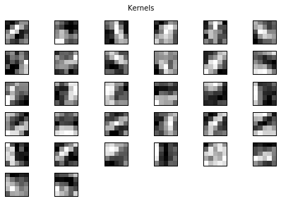
We can visualize the 32 kernels the network learned for convolution layer 1. Each kernel is capturing an important element of a handwritten digit, which can be combined through later layers to form each of the 0-9 digits:
c1_kernels = weights[0]  # get the learned weights for the first conv layer

fig = plt.figure()
fig.suptitle("Kernels")

for j in range(len(c1_kernels)):
    ax = fig.add_subplot(6, 6, j+1)
    ax.matshow(c1_kernels[j][0], cmap=cm.gray)
    plt.xticks(np.array([]))
    plt.yticks(np.array([]))

plt.show()
They may look somewhat random at first glance, but we can see that clear structure being learned in most kernels. For example, kernels 3 and 4 seem to be learning diagonal edges in opposite directions, and other capture round edges or enclosed spaces:
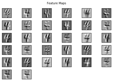
We can also take a single training example and convolve each kernel over the digit to see the feature maps, which shows the areas of the input that are being activated by that kernel. Kernels and feature maps for later convolution layers cannot be visualized easily because they don’t operate directly on the input images – their input is dependent on the output of the previous layer. We can directly visualize the C1 level feature maps for a single random training image:
image_num = np.random.randint(0, X_train.shape[0])
image_array = X_train[image_num][0]
image_2d = np.reshape(image_array, (28, 28))
image_4d = image_2d.reshape(1, 1, 28, 28)  # 4D representation of the image

x = T.tensor4().astype(theano.config.floatX)
conv_out = T.nnet.conv2d(input=x, filters=c1_kernels)  # convolve each kernel over the image

get_activity = theano.function([x], conv_out)
activation = get_activity(image_4d)

fig = plt.figure()
fig.suptitle("Feature Maps")

for j in range(len(c1_kernels)):
    ax = fig.add_subplot(6, 6, j+1)
    ax.matshow(activation[0][j], cmap=cm.gray)
    plt.xticks(np.array([]))
    plt.yticks(np.array([]))

plt.show()
In summary, CNNs can learn the visual structure of images and learn to identify the features that distinguish one number from another. This idea can be extended to colour images pretty easily (for example with the CIFAR-10 dataset), or even non-image-based inputs as long as there’s some spatial structure inherent in the input.
As always, the full code for this example can be found in my GitHub repo here.