We previously talked about Convolutional Neural Networks (CNN) and how use them to recognize handwritten digits using Lasagne. While we can manually extract kernel parameters to visualize weights and activation maps (as discussed in the previous post), the nolearn package offers an easy way to visualize different elements of CNNs.
nolearn is a wrapper around Lasagne (which itself is a wrapper around Theano), and offers some nice visualization options such as plotting occlusion maps to help diagnose the performance of a CNN model. Additionally, nolearn offers a very high level API that makes model training even simpler than with Lasagne.
In this short post I’ll go through how to train a simple CNN model using nolearn for the task of recognizing handwritten digits (MNIST database). You will need nolearn, Lasagne, and Theano.
To start, we need to import a number of layer modules from Lasagne, as well as visualization modules from nolearn:
from __future__ import print_function

import sys
import os
import numpy as np

from lasagne.layers import DenseLayer
from lasagne.layers import InputLayer
from lasagne.layers import DropoutLayer
from lasagne.layers import Conv2DLayer
from lasagne.layers import MaxPool2DLayer
from lasagne.nonlinearities import softmax
from lasagne.updates import nesterov_momentum

from nolearn.lasagne import NeuralNet
from nolearn.lasagne import TrainSplit
from nolearn.lasagne.visualize import plot_loss
from nolearn.lasagne.visualize import plot_conv_weights
from nolearn.lasagne.visualize import plot_conv_activity
from nolearn.lasagne.visualize import plot_occlusion
Like before we need to load the MNIST data using the function supplied by the Lasagne tutorial:
def load_dataset():
    # We first define a download function, supporting both Python 2 and 3.
    if sys.version_info[0] == 2:
        from urllib import urlretrieve
    else:
        from urllib.request import urlretrieve

    def download(filename, source='http://yann.lecun.com/exdb/mnist/'):
        print("Downloading %s" % filename)
        urlretrieve(source + filename, filename)

    # We then define functions for loading MNIST images and labels.
    # For convenience, they also download the requested files if needed.
    import gzip

    def load_mnist_images(filename):
        if not os.path.exists(filename):
            download(filename)
        # Read the inputs in Yann LeCun's binary format.
        with gzip.open(filename, 'rb') as f:
            data = np.frombuffer(f.read(), np.uint8, offset=16)
        # The inputs are vectors now, we reshape them to monochrome 2D images,
        # following the shape convention: (examples, channels, rows, columns)
        data = data.reshape(-1, 1, 28, 28)
        # The inputs come as bytes, we convert them to float32 in range [0,1].
        # (Actually to range [0, 255/256], for compatibility to the version
        # provided at http://deeplearning.net/data/mnist/mnist.pkl.gz.)
        return data / np.float32(256)

    def load_mnist_labels(filename):
        if not os.path.exists(filename):
            download(filename)
        # Read the labels in Yann LeCun's binary format.
        with gzip.open(filename, 'rb') as f:
            data = np.frombuffer(f.read(), np.uint8, offset=8)
        # The labels are vectors of integers now, that's exactly what we want.
        return data

    # We can now download and read the training and test set images and labels.
    X_train = load_mnist_images('train-images-idx3-ubyte.gz')
    y_train = load_mnist_labels('train-labels-idx1-ubyte.gz')
    X_test = load_mnist_images('t10k-images-idx3-ubyte.gz')
    y_test = load_mnist_labels('t10k-labels-idx1-ubyte.gz')

    # We just return all the arrays in order, as expected in main().
    # (It doesn't matter how we do this as long as we can read them again.)
    return X_train, y_train, X_test, y_test

# Load MNIST data
X_train, y_train, X_test, y_test = load_dataset()
Setting up the network architecture using nolearn is extremely straightforward, we simply define the layers (and their associated parameters) using a list:
layers0 = [
    # layer dealing with the input data
    (InputLayer, {'shape': (None, X_train.shape[1], X_train.shape[2], X_train.shape[3])}),

    # first stage of our convolutional layers
    (Conv2DLayer, {'num_filters': 32, 'filter_size': (5,5)}),
    (MaxPool2DLayer, {'pool_size': (2,2)}),

    # second stage of our convolutional layers
    (Conv2DLayer, {'num_filters': 32, 'filter_size': (3,3)}),
    (MaxPool2DLayer, {'pool_size': (2,2)}),

    # two dense layers with dropout
    (DenseLayer, {'num_units': 64}),
    (DropoutLayer, {}),
    (DenseLayer, {'num_units': 64}),

    # the output layer
    (DenseLayer, {'num_units': 10, 'nonlinearity': softmax}),
]
Then we specify the learning-related parameters for our model, such as the number of epochs, learning rate, and regularization. We also have to pass in the layers that we previously defined:
net0 = NeuralNet(
    layers=layers0,
    max_epochs=3,

    update=nesterov_momentum,
    update_learning_rate=0.1,
    update_momentum=0.9,

    objective_l2=0.0025,

    train_split=TrainSplit(eval_size=0.25),
    verbose=2,
)
With that, our model is ready to go! To train it we simply call the fit method with our training data:
net0.fit(X_train, y_train)
Visualization options
Whereas in previous posts we had to manually save and plot our training curves, nolearn has a function to directly plot the training and validation loss values over epochs:
plot_loss(net0)
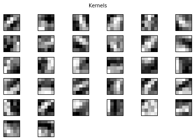
We can plot the learned kernels for any layer in the network:
plot_conv_weights(net0.layers_[1], figsize=(4, 4)) # Layer 1 (conv1)
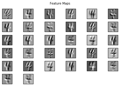
We can also plot the activation/feature maps for a single image:
x = X_train[0:1]  # training image
plot_conv_activity(net0.layers_[1], x)
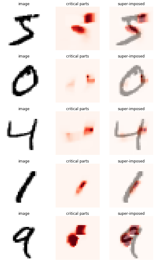
One of the nicest features offered by nolearn is plotting occlusion maps. Occlusion maps are created by occluding parts of the image and seeing how that affects the predictive power of the model. The critical parts of the image are the areas that are important for correct prediction:
plot_occlusion(net0, X_train[:5], y_train[:5])
There are other visualization options available such as drawing the network architecture (draw_to_notebook(net0)) and saliency maps (plot_saliency(net0, X_train[:5]). You can explore some of these other options in the nolearn tutorial here. Overall, nolearn is great as it provides the ability to visualize different aspects of the learned model without too much manual work.