So far we have extracted webcam features and collected coordinate data. Now we can use that dataset to create our deep learning model with PyTorch. The following models and analyses were conducted in a Jupyter notebook, which can be found here.
The problem we have is basically bounding box regression, but simplified to only 2 continuous output values (X-Y screen coordinate). To summarize, the data we have available to us:
- Possible inputs
- Unaligned face (3D Image)
- Aligned face (3D Image)
- Left eye (3D Image)
- Right eye (3D Image)
- Head position (2D Image)
- Head angle (Scalar)
- Outputs
- X screen coordinate
- Y screen coordinate
The goal is to find the most accurate model that can map some combination of inputs to an output X-Y coordinate pair. We will be experimenting with a few different models to find the best fit.
We will be using Mean Squared Error (MSE) as our loss function. When it comes to the “real world” accuracy of our model, we will take the square root of that (RMSE). This can be interpreted as the pixel-wise distance between our predicted location and the true location. For example, an MSE loss value of 10,000 would be equivalent to 100 pixels of inaccuracy in the prediction.
Dataset overview
The dataset contains 25,738 examples, with 69.01% of screen locations being sampled at least once. The entire dataset is 319MB in size.
The first thing we can do is check how that dataset is distributed across the screen:
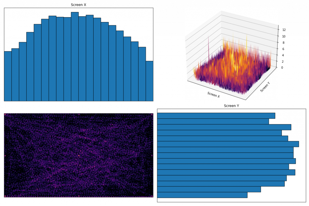
In the bottom-left and top-right, you can see a 2D and 3D plot of the region map we created, which shows the number of data samples at each region of the screen.
In the top-left and bottom-right are histograms showing the number of samples within each section of the screen. As suspected, the center of the screen contains the most data samples, with the edges being relatively under sampled. This may end up reducing prediction accuracy near the edges and corners.
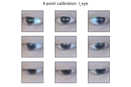
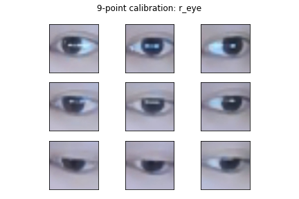
For those extreme screen regions, we can check to make sure there is good variation in input features. For example, we can see there is a difference in the way the eyes look when they are gazing at the 9 calibration locations:
Ingesting data
We first need a way to get our data into our models. For that we can use PyTorch Dataset and DataLoader. These allow us to define how data samples are retrieved from disk, and handles preprocessing, shuffling, and batching of the data. The benefit is that we don’t need to load the entire dataset into memory – data batches are loaded as needed.
PyTorch Dataset
For the Dataset, we can define where the data is stored in the __init__ method. Then the __getitem__ method defines what should happen when our DataLoader makes a request for data. In this case it simply uses PIL to load the image and applies a few image transformations:
import pandas as pd
import torch
from torch.utils.data import Dataset
from torchvision import transforms
from PIL import Image

class FaceDataset(Dataset):
    def __init__(self, cwd, data_partial, *img_types):
        if data_partial:
            self.dir_data = cwd / "data_partial"
        else:
            self.dir_data = cwd / "data"

        df = pd.read_csv(self.dir_data / "positions.csv")
        df["filename"] = df["id"].astype("str") + ".jpg"

        self.img_types = list(img_types)
        self.filenames = df["filename"].tolist()
        self.targets = torch.Tensor(list(zip(df["x"], df["y"])))
        self.head_angle = torch.Tensor(df["head_angle"].tolist())

        self.transform = transforms.Compose(
            [transforms.ColorJitter(brightness=0.3, contrast=0.3, saturation=0.3, hue=0.1),
             transforms.ToTensor()]
        )

    def __len__(self):
        return len(self.targets)

    def __getitem__(self, idx):
        batch = {"targets": self.targets[idx]}

        if "head_angle" in self.img_types:
            batch["head_angle"] = self.head_angle[idx]

        for img_type in self.img_types:
            if not img_type == "head_angle":
                img = Image.open(self.dir_data / f"{img_type}" / f"{self.filenames[idx]}")
                if img_type == "head_pos":
                    # Head pos is a generated black/white image and shouldn't be augmented
                    img = transforms.ToTensor()(img)
                else:
                    img = self.transform(img)
                batch[img_type] = img

        return batch
PyTorch DataLoader
The DataLoader handles the task of actually getting a batch of data and passing it to our PyTorch models. Here you can control things like the batch size and whether the data should be shuffled. I created a function to split my entire dataset into train/validation/test sets, and creates a DataLoader for each:
def create_datasets(cwd, data_partial, img_types, batch_size=1, train_prop=0.8, val_prop=0.1, seed=87):
    dataset = FaceDataset(cwd, data_partial, *img_types)
    n_train = int(len(dataset) * train_prop)
    n_val = int(len(dataset) * val_prop)
    n_test = len(dataset) - n_train - n_val
    ds_train, ds_val, ds_test = random_split(
        dataset, (n_train, n_val, n_test), generator=torch.Generator().manual_seed(seed)
    )

    train_loader = DataLoader(ds_train, batch_size=batch_size, shuffle=True, pin_memory=True)
    val_loader = DataLoader(ds_val, batch_size=batch_size, shuffle=False, pin_memory=True)
    test_loader = DataLoader(ds_test, batch_size=batch_size, shuffle=False, pin_memory=True)

    return train_loader, val_loader, test_loader
Face model
We’ll start by creating a simple model using only the unaligned face image. We can use PyTorch Lightning for this as it helps to streamline the code and remove a lot of boilerplate.
PyTorch Lightning
First, we create a LightningModule, which is where we define the layers in the model (__init__) and what happens during a single forward pass (forward). This receives a config object, which contains a number of hyperparameters that we will be tuning (more on this in the next section):
class SingleModel(pl.LightningModule):
    def __init__(self, config, img_type):
        super().__init__()
        self.save_hyperparameters()  # stores hparams in saved checkpoint files

        feat_size = 64
        self.example_input_array = torch.rand(1, 3, feat_size, feat_size)

        self.img_type = img_type
        self.lr = config["lr"]
        self.filter_size = config["filter_size"]
        self.filter_growth = config["filter_growth"]
        self.n_filters = config["n_filters"]
        self.n_convs = config["n_convs"]
        self.dense_nodes = config["dense_nodes"]

        # First layer after input
        self.conv_input = nn.Conv2d(3, self.n_filters, self.filter_size)
        feat_size = feat_size - (self.filter_size - 1)

        # Additional conv layers
        self.convs1 = nn.ModuleList()
        n_out = self.n_filters
        for i in range(self.n_convs):
            n_in = n_out
            n_out = n_in * self.filter_growth

            self.convs1.append(self.conv_block(n_in, n_out, self.filter_size))
            # Calculate input feature size reductions due to conv and pooling
            feat_size = (feat_size - (self.filter_size - 1)) // 2

        # FC layers -> output
        self.drop1 = nn.Dropout(0.2)
        self.fc1 = nn.Linear(n_out * feat_size * feat_size, self.dense_nodes)
        self.drop2 = nn.Dropout(0.2)
        self.fc2 = nn.Linear(self.dense_nodes, self.dense_nodes // 2)
        self.fc3 = nn.Linear(self.dense_nodes // 2, 2)

    def forward(self, x):
        x = self.conv_input(x)
        for c in self.convs1:
            x = c(x)

        x = x.reshape(x.shape[0], -1)
        x = self.drop1(F.relu(self.fc1(x)))
        x = self.drop2(F.relu(self.fc2(x)))
        x = self.fc3(x)
        return x

    def conv_block(self, input_size, output_size, filter_size):
        block = nn.Sequential(
            OrderedDict(
                [
                    ("conv", nn.Conv2d(input_size, output_size, filter_size)),
                    ("relu", nn.ReLU()),
                    ("norm", nn.BatchNorm2d(output_size)),
                    ("pool", nn.MaxPool2d((2, 2))),
                ]
            )
        )
        return block
The unaligned face image is first passed through a convolution layer. That’s followed by a number of “convolution blocks”, which consists of convolution, ReLu activation, batch normalization, and max pooling. The output from these blocks is then resized and passed into some fully connected layers with dropout.
A few things to note:
- Calling
save_hyperparameters()is not required, but it allows us to log the hyperparameters being used in this model for reference and for Tensorboard - The
self.example_input_arrayattribute is a blank input tensor, and is required for logging the graph to Tensorboard
The class also needs methods that define what happens during each step of training/validation/test. You can find the full class here.
Next, we have a function that creates our dataset, instantiates our model, creates a trainer, and fits the model:
def train_single(
    config,
    cwd,
    data_partial,
    img_types,
    num_epochs=1,
    num_gpus=-1,
    save_checkpoints=False,
):
    d_train, d_val, d_test = create_datasets(cwd, data_partial, img_types, seed=config["seed"], batch_size=config["bs"])
    model = SingleModel(config, *img_types)

    trainer = pl.Trainer(
        max_epochs=num_epochs,
        gpus=num_gpus,
        accelerator="dp",
        progress_bar_refresh_rate=0,
        checkpoint_callback=save_checkpoints,
        logger=TensorBoardLogger(save_dir=tune.get_trial_dir(), name="", version=".", log_graph=True),
        callbacks=[TuneReportCallback({"loss": "val_loss"}, on="validation_end")],
    )

    trainer.fit(model, train_dataloader=d_train, val_dataloaders=d_val)
Ray Tune
Finally, we need to wrap the training function in some Ray Tune code that allows us to do hyperparameter tuning. Ray Tune provides an extremely simple way to do (distributed) hyperparameter tuning. One of the best things about Ray Tune is that it offers an algorithm called ASHA.
Traditionally, when you tune hyperparameters using grid search or random search, you fully train all of your model/hyperparameters combinations. This can be a waste of resources, because you can tell early on that some models just won’t work well. ASHA is a halving algorithm that prunes poor performing models, and only full trains the best models.
def tune_asha(
    config,
    train_func,
    name,
    img_types,
    num_samples,
    num_epochs,
    data_partial=False,
    save_checkpoints=False,
    seed=1,
):
    cwd = Path.cwd()

    scheduler = ASHAScheduler(max_t=num_epochs, grace_period=1, reduction_factor=2)

    reporter = JupyterNotebookReporter(
        overwrite=True,
        parameter_columns=list(config.keys()),
        metric_columns=["loss", "training_iteration"],
    )

    analysis = tune.run(
        tune.with_parameters(
            train_func,
            cwd=cwd,
            data_partial=data_partial,
            img_types=img_types,
            save_checkpoints=save_checkpoints,
            num_epochs=num_epochs,
            num_gpus=1,
        ),
        resources_per_trial={"cpu": 2, "gpu": 1},
        metric="loss",
        mode="min",
        config=config,
        num_samples=num_samples,
        scheduler=scheduler,
        progress_reporter=reporter,
        name="{}/{}".format(
            name, datetime.datetime.now().strftime("%Y-%b-%d %H-%M-%S")
        ),
        local_dir=cwd / "logs"
    )
Training the unaligned face model
With all the helper functions defined, training the model is as simple as providing a range of hyperparameter values as a config dictionary, and calling our tune function. PyTorch also allows us to log training results to Tensorboard for analysis.
We start by exploring a wide range of values to get a sense of what the search space looks like:
config = {
        "seed": tune.randint(0, 10000),  # reproducible random seed for each experiment
        "bs": tune.choice([1 << i for i in range(2, 9)]),  # batch size
        "lr": tune.loguniform(1e-7, 1e-3),  # learning rate
        "filter_size": tune.choice([3, 5, 7, 9]),  # filter size (square)
        "filter_growth": tune.choice([1, 2]),  # increase filter count by a factor
        "n_filters": tune.choice([8, 16, 32, 64]),  # number of starting filters
        "n_convs": tune.choice([0, 1, 2]),  # number of conv layers
        "dense_nodes": tune.choice([16, 32, 64, 128]),  # number of nodes in fc layer
    }

analysis = tune_asha(config, data_partial=True, train_func=train_single, name="face/explore", img_types=["face"], num_samples=100, num_epochs=10, seed=87)
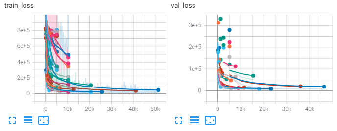
If we look at the train and validation graphs, we can see ASHA in action. ASHA prunes poorly performing models to save time:
We can then check hyperparameter performance in Tensorboard to get a sense of how we can narrow the ranges:
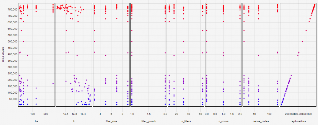
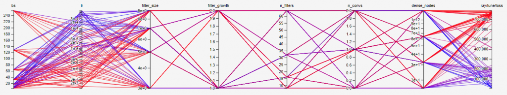
For example, we can see that the best performing models (coloured blue) tend to have small batch sizes, learning rate around 1×10⁻⁴, and a larger number of fully connected (dense) nodes. We can use this information to fine tune the hyperparameter ranges and search again over more epochs.
After a second round of search, we take the best performing hyperparameters and train the final model over 50 epochs:
start_time = datetime.datetime.now().strftime("%Y-%b-%d %H-%M-%S")

config = get_best_results(Path.cwd()/"logs"/"face"/"tune")

pl.seed_everything(config["seed"])

d_train, d_val, d_test = create_datasets(Path.cwd(), data_partial=True, img_types=["face"], seed=config["seed"], batch_size=config["bs"])

model = SingleModel(config, "face")
trainer = pl.Trainer(
    max_epochs=50,
    gpus=[0, 1],
    accelerator="dp",
    checkpoint_callback=True,
    logger=TensorBoardLogger(save_dir=Path.cwd()/"logs", name="face/final/{}".format(start_time), log_graph=True))

trainer.fit(model, train_dataloader=d_train, val_dataloaders=d_val)

test_results = trainer.test(test_dataloaders=d_test)
On the test set we get an MSE loss of 2362, which is a pixel error of around 48.6 pixels.
We can use the same functions to compare the face model to one using the aligned face images instead. You can find the details of this process in the Jupyter notebook. The aligned face model gives a larger MSE loss of 2539, and a pixel error of 50.4 pixels.
The performance with aligned faces is slightly worse. It’s possible that head angle is an important feature for eye tracking, and is being learned indirectly from the unaligned face image through multiple convolutions.
Eye model
For an eye tracker, it’s a good idea to check a model where we only input the eye images.
This is slightly more complicated as we have 2 input images, but we just need to add a second network of convolutions, and merge the results from the left and right eye image convolutions before going into the fully connected layers. You can find the full model definition here.
After going through the same process of exploring initial hyperparameter ranges, fine tuning the values, and fully training the best model of 50 epochs, we get an MSE loss of 3837, and a pixel error of 61.9 pixels.
Using eye image inputs appears to result in a model that is significantly worse than using the face image alone. Presumably this is because the face image already contains both eyes, and is able to isolate those regions through successive convolutions.
Multiple input model
To recap the performance of our models:
- Unaligned face: 48.6 pixel error
- Aligned face: 50.4 pixel error
- Eyes: 61.9 pixel error
So far, our best performing model uses a single unaligned face image. Next, we need to test more complex models that use combinations of these different images. I suspect that a full face image provides most of the information needed, but passing the eyes separately would help the model focus on those regions specifically. We can also pass in head angle and head position, which would allow us to keep the face network relatively shallow.
The plan is to use the unaligned face, left and right eye, head position, and head angle as inputs into the same model. Each of these features will be passed into a “sub” network of the model. We will also allow each one to take on different hyperparameter values (e.g., filter size, layer depth etc.).
Unknown sizes
This is the point in my PyTorch learning where I hit my only real difficulty. Each image input will pass through a different number of convolution/pool layers, using different number of kernels, with different layers sizes. If we plan on tuning each of these as separate parameters, then we cannot determine ahead of time what the final size post-convolution will be. Hence, we won’t know how many input nodes the fully connected layer needs.
You will need to manually track and calculate feature map sizes, for each image, after an undetermined number of convolution/pooling operations. This proved to be a bit of a headache as PyTorch requires layer dimensions to be defined in the __init__ method of the class. Doing this manually took over 100 lines of code. If someone knows of an automatic way to do this then please let me know!
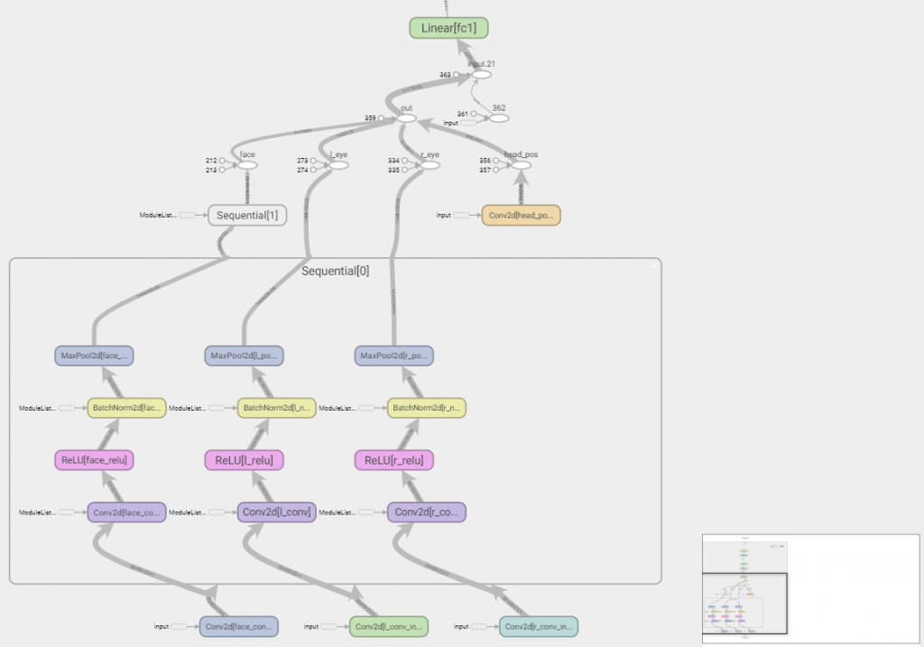
The final model
After going through the hyperparameter exploration/tuning/finalization process, the best performing model had the following architecture:
- Unaligned face:
- Convolution
- Block: (convolution + ReLu + batch norm + max pool)
- Block: (convolution + ReLu + batch norm + max pool)
- Left eye
- Convolution
- Block: (convolution + ReLu + batch norm + max pool)
- Right eye
- Convolution
- Block: (convolution + ReLu + batch norm + max pool)
- Head position
- Convolution
- The outputs of each of the sub-networks above are merged with head angle
- Everything is then flattened -> 128 node fully connected layer -> 64 fully connected layer
   | Name                   | Type        | Params | In sizes         | Out sizes
----------------------------------------------------------------------------------------------
   | face_conv_input        | Conv2d      | 4.7 K  | [1, 3, 64, 64]   | [1, 32, 58, 58]
   | face_convs.0.face_conv | Conv2d      | 100 K  | [1, 32, 58, 58]  | [1, 64, 52, 52]
   | face_convs.0.face_relu | ReLU        | 0      | [1, 64, 52, 52]  | [1, 64, 52, 52]
   | face_convs.0.face_norm | BatchNorm2d | 128    | [1, 64, 52, 52]  | [1, 64, 52, 52]
   | face_convs.0.face_pool | MaxPool2d   | 0      | [1, 64, 52, 52]  | [1, 64, 26, 26]
   | face_convs.1.face_conv | Conv2d      | 401 K  | [1, 64, 26, 26]  | [1, 128, 20, 20]
   | face_convs.1.face_relu | ReLU        | 0      | [1, 128, 20, 20] | [1, 128, 20, 20]
   | face_convs.1.face_norm | BatchNorm2d | 256    | [1, 128, 20, 20] | [1, 128, 20, 20]
   | face_convs.1.face_pool | MaxPool2d   | 0      | [1, 128, 20, 20] | [1, 128, 10, 10]

   | l_conv_input           | Conv2d      | 2.4 K  | [1, 3, 64, 64]   | [1, 32, 60, 60]
   | l_convs.0.l_conv       | Conv2d      | 51.3 K | [1, 32, 60, 60]  | [1, 64, 56, 56]
   | l_convs.0.l_relu       | ReLU        | 0      | [1, 64, 56, 56]  | [1, 64, 56, 56]
   | l_convs.0.l_norm       | BatchNorm2d | 128    | [1, 64, 56, 56]  | [1, 64, 56, 56]
   | l_convs.0.l_pool       | MaxPool2d   | 0      | [1, 64, 56, 56]  | [1, 64, 28, 28]

   | r_conv_input           | Conv2d      | 2.4 K  | [1, 3, 64, 64]   | [1, 32, 60, 60]
   | r_convs.0.r_conv       | Conv2d      | 51.3 K | [1, 32, 60, 60]  | [1, 64, 56, 56]
   | r_convs.0.r_relu       | ReLU        | 0      | [1, 64, 56, 56]  | [1, 64, 56, 56]
   | r_convs.0.r_norm       | BatchNorm2d | 128    | [1, 64, 56, 56]  | [1, 64, 56, 56]
   | r_convs.0.r_pool       | MaxPool2d   | 0      | [1, 64, 56, 56]  | [1, 64, 28, 28]

   | head_pos_conv_input    | Conv2d      | 160    | [1, 1, 64, 64]   | [1, 16, 62, 62]

   | drop1                  | Dropout     | 0      | [1, 128]         | [1, 128]
   | fc1                    | Linear      | 22.4 M | [1, 174657]      | [1, 128]
   | drop2                  | Dropout     | 0      | [1, 64]          | [1, 64]
   | fc2                    | Linear      | 8.3 K  | [1, 128]         | [1, 64]
   | fc3                    | Linear      | 130    | [1, 64]          | [1, 2]
----------------------------------------------------------------------------------------------
23.0 M    Trainable params
The model appears to perform best when the face image is passed through 2 full convolution blocks with a large filter size of 7×7. While head position (being only a 2D image) only requires a single convolution layer with a small filter size of 3×3.
When we pass the test set through this model, we get an MSE loss of 2037, and a pixel error of 45.1 pixels. This is the best performing model so far.
Errors over screen space
The pixel error values we’ve been looking at are averaged over the entire screen. This is useful for comparing models, but not so useful for determining if there are certain screen locations where our model performs poorly.
What we can do is plot the prediction error at each coordinate of the screen to see if there are any patterns. The functions for this are predict_screen_error and plot_screen_errors. They return a plot of errors over screen space.
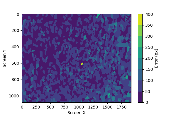
In the case of the full model with multiple inputs, the error map looks like this:
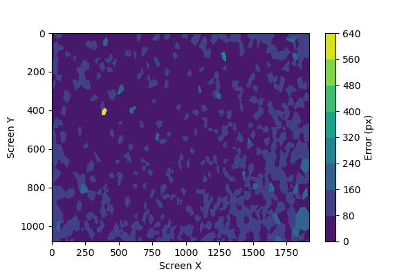
What we can see, as suspected based on the original distribution of collected data, is that the screen edges and corners tend to have the highest prediction errors.
We can try to improve this by collecting more data, and prioritizing screen edges using the flags in config.ini. When we double the dataset to 50k samples and retrain the same model, we end up with a pixel error of 48.4px.
The average pixel error is slightly worse than our previous attempt, but if we look at the error map we can see that the errors are smaller and more diffused across the entire screen:
Of course, there are more models we can test and we can find other ways to improve our prediction accuracy. But at this point we can try deploying it into a test application to see how well it works. See you in the next post.